Random forests for tracking in ultrasonic images

MICCAI CLUST is a challenge for tracking objects in medical ultrasonic image sequences, which move back and forth along a specific trajectory, often (but not necessarily) in periodical turns. Amongst other influences, the major difficulties are the variations of the object's appearance and shape, already after a few frames.

For this purpose, two different machine learning algorithms are presented in the following, as part of the master thesis.

Description

leo

Both are based on random forest, a method that is known for its good accuracy and also for its good generalization capabilities. The classifier in the one approach is used for pixel classification (object and environment), where the actual position is given as an output according to the estimated object elements. In the other algorithm, the forest is used as a landmark estimation, that retrieves the current position on an initially learned trajectory. The latter idea has been submitted to and evaluated by CLUST.

Both algorithms share the following attributes:

• No external dataset is required, the algorithm creates it online and autonomously.
• After the hyper parameter tuning, the user is only required to initially select an appropriate object even when switching the scanner device (i.e. plug-and-play).
• Good tracking accuracy.

1^st algorithm: pixel classification

With this method, simply a black image is desired, were only the object is highlighted. By this definition, a binary image is generated, where the individual highlighted pixel collectively provide the information about the object's position on the current frame. For this purpose, a dataset is necessary to train the random forest. This is done in two steps: generating the labels and afterwards extracting the feature vectors.

Since CLUST15 does not provide any further dataset information, except for an object position annotation for just a few frames, the labels need to be generated artificially. Therefore, when the user selects the initial tracking center, all adjacent pixels are identified as object (white) when their intensity levels are within a certain tolerance band, which is related to the intensity levels around the object's center. All remaining pixels are labeled as environment (black).This first step is visualized in the image below.

Subsequently, the features are generated (e.g.: mean filter, local maximum or minimum). A feature vector is then generated when for a certain coordinate all feature responses are extracted in a fixed order. The actual dataset is then generated, when the labels from step 1 are combined with the so extracted vectors:

The forest is trained afterwards. The procedures during the testing phase are basically: receive new frame, extract features, estimate pixel identities, binarize the image and finally extract the object's position. For the last step multiple center definitions could be utilized. In this case, a poor estimate is shown in the picture above. In step 4 on this image, the pixel estimation shows the output of the random forest (how likely a given pixel is part of the object), where the extracted object shows the desired binarized image. The mean position (marked as the yellow cross) retrieves a less accurate result, more appropriate for instance would be the coordinates of the centroid.

Additional attributes of this approach are:

• Usually adapts well to new circumstances (since it relies on the feature responses and not the object's changing appearance).
• An arbitrary kind of center definition can be chosen (e.g.: mean, centroid).
• Tends to lose the object over time.
• Previous results could spoil subsequent estimates (in case the object is getting lost).

2^nd algorithm: landmark estimation

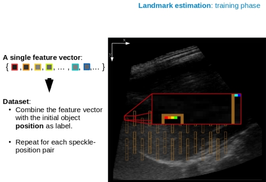
This method is designed to catch the drawbacks from the pixel classification, but it is based on a completely different approach, where occurring wave interferences give information about the current position.

Waves are observable on different media, for instance: water, light or sound. They are known for the fact, whenever multiple waves intersect at a certain point, then their amplitudes add up and thus often either increase or decrease the level of the resulting amplitude. This phenomenon also occurs on ultrasound images, where it is known as speckle patterns that take influence on particular pixel intensities individually. It causes on the image a similar appearance as salt-and-pepper noise. Most importantly, they come with the attribute that these patterns are reproducible. Since an object moves back and forth on a trajectory, this fact could be used to match a speckle appearance with a certain position on the object's trajectory. But to reproduce the exact same speckle appearance, the whole situation needs to be reproduced (which includes for instance: the pose of the scanner's head, pose of the bones and tissues from where the sound wave was reflected). Of course, a full reconstruction of a former case is an ideal state, because all involved elements vary a little over time, for which a machine learning method is required, that generalizes well and thus is capable to catch this variations.

At first the trajectory needs to be recorded, which can be achieved within very few breathing cycles (usually after 2-3 cycles). Therefore, with the help of the correlation coefficient, the object is tracked on the initial frames. During this time, the information is stored for generating the dataset, because on the one hand the object's position are simply used as labels and on the other hand, for each position, the current pixel intensities are extracted from a fixed area, as the dataset's feature vector. The following image illustrates the generation of the dataset.

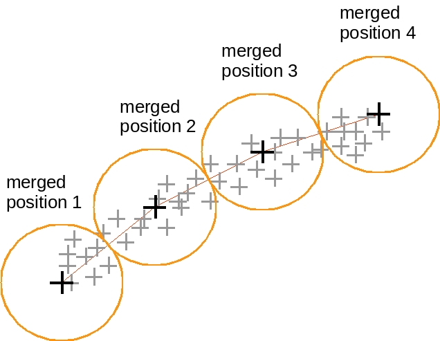
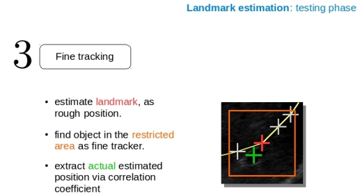
Brown boxes show the area where the pixel intensities are extracted (influenced by the speckle phenomenon), the bigger red box indicates a magnified version of the smaller red one. The first feature of the vector, is the pixel indicated by the red square, the second feature is the orange square, the yellow as third and the green as the fourth feature of the vector. The blue marked pixels are used too, but just at a later position, because they are extracted from a different box. In other words for this setting, the length of this vector is > 1000 Features.

At this point there is only a dataset with 200 entries (when 200 frames were used as initial run), with 200 individual labels and very large feature vectors. To increase the dataset quality, the labels (or landmarks) can be merged, so more vectors are available for less labels, with the drawback only a rough position can be estimated. Therefore a subsequent fine tracker, which retrieves the exact position needs to be applied. For this the correlation coefficient was also utilized to find the object within a constricted area around the rough position estimate.

Additional attributes for this method are:

• Real time processing is feasible.
• Independent from previous results and frame-consecutiveness.
• Tracker does not lose the object in the same manner the first algorithm does, as long as the trajectory was successfully trained.
• Tracks arbitrary features (if it is recognizable for the fine tracker).
• Object needs to move along the learned trajectory.

Results

Because the landmark estimation was more robust, it is the chosen algorithm which was submitted to the CLUST challenge in march 2017. After parameter tuning, the algorithm's tracking capabilities was evaluated by the challenge maintainers themselves. The euclidean error distance between estimated and annotated object position for all sequences of the test set are listed in the following table.

CLUST15 test set evaluation:

For comparison, all published results from other participants can be found here.

Files

Full version of the master thesis

Here is a video that illustrates both algorithms. For the pixel classification, only the frames with the annotated position were taken, which are in order but non-consecutive, thus this part appears laggy. The second part demonstrates the situation, where the algorithm of the landmark estimation enlarges the trajectory, to continue estimating the right position when the initial trained circumstances varied. Since this video was created independently for each sequence, the actual processing speed is not shown.

License

This original work is copyright by University of Bremen.
Any software of this work is covered by the European Union Public Licence v1.2. To view a copy of this license, visit eur-lex.europa.eu.
The Thesis provided above (as PDF file) is licensed under Attribution-NonCommercial-NoDerivatives 4.0 International.
Any other assets (3D models, movies, documents, etc.) are covered by the Creative Commons Attribution-NonCommercial-ShareAlike 4.0 International License. To view a copy of this license, visit creativecommons.org.
If you use any of the assets or software to produce a publication, then you must give credit and put a reference in your publication.
If you would like to use our software in proprietary software, you can obtain an exception from the above license (aka. dual licensing). Please contact zach at cs.uni-bremen dot de.