Motivation

1. Dickerson, Duncan, Goodrich: K-D Trees are Better when Cut on the Longest Side; ESA 2000 (LNCS 1879)
2. Arya, Mount, Netanyahu, Silverman, Wu: An Optimal Algorithm for Approximate Nearest Neighbor Searching in Fixed Dimensions; Journal of the ACM, Volume 45 Issue 6, Nov. 1998

The "(1+ε)-nearest neighbor" of a query point q is a point p^o ∈ S, such that || p^o - q || ≤ (1+ε) || p^* - q ||. Such a point p^o is called an "approximate nearest neighbor" to q (there might be many).

The "standard approximate nearest-neighbor search algorithm" is as follows (in Python):

    def approx_nn( self, query, epsilon ):
        cell_region = self._cell_region                         # root cell region
        queue = []                                              # p-queue of nodes, sorted by distance to query
        node = self
        current_nn = None                                       # current candidate for NN, 
        current_d = sys.float_info.max                          # start with "infinite" point

        while cell_region.dist(query) < current_d/(1.0 + epsilon):

            # descend into closest leaf
            while node._split_axis is not None:
                left_region, right_region = cell_region.split( node._split_axis, node._split_value )
                dl = left_region.dist( query )
                dr = right_region.dist( query )
                if dl < dr:                                     # left child is closer
                    heappush( queue, (dr, node._right, right_region) )
                    node = node._left
                    cell_region = left_region
                else:                                           # right child is closer
                    heappush( queue, (dl, node._left, left_region) )
                    node = node._right
                    cell_region = right_region

            # we are now at a leaf
            d = query.dist( node._point )
            if d < current_d:
                current_nn = node._point
                current_d = d

            if not queue:
                break                                           # last node was processed

            # process next node, which is the closest of all unprocessed yet
            dn, node, cell_region = heappop( queue )
        # end while

        return current_d, current_nn
    # end def approx_nn

One reason for my experiments was that Dickerson, Duncan, and Goodrich show in their paper that this standard algorithm, when used on "longest side" kd-trees, has a worst-case complexity of O( ¹⁄_ε^d-1 log^d n ). So I wanted to see, how bad the influence of the ε really is, and what other "hidden" constants there might be in the Big-O.

Another reason was that a lot of people seem to use the ANN Library, developed by Mount and Arya. However, the data structure used in that library (AFAIK) is a much more complicated variant of kd-trees, which they call BBD-tree (many people seem to call it "ANN kd-tree", which makes no sense). And since they have provided the results of some experiments with their BBD-trees in their paper, I wanted to see whether or not the standard (i.e., "longest side") kd-trees would perform as well.
It would be interesting to see how many leaves a typical ANN search using BBD-trees visits, but I doubt that they give a substantial performance gain. (Please share any experience you might have with me.)

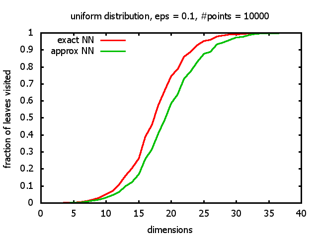
And yet another reason was that I wanted to see for myself at which point the "curse of dimensionality" begins to exert its influence in the case considered here.

The Experiments

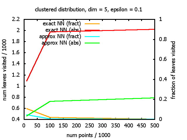
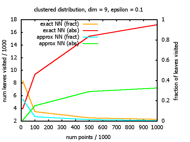
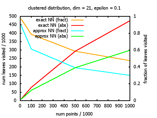
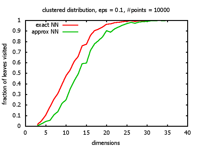
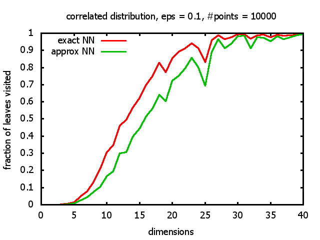
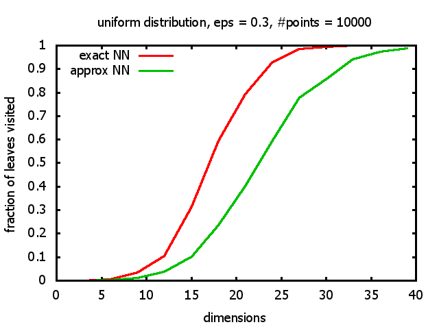
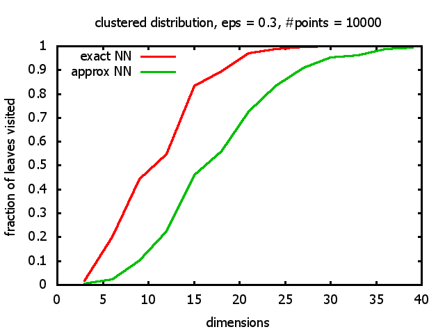
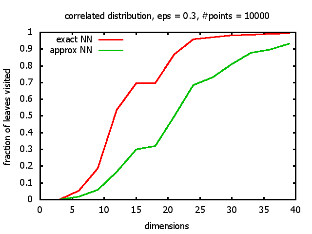
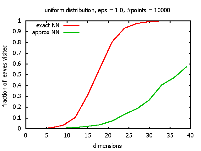
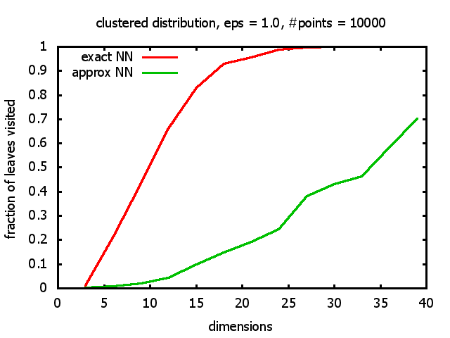
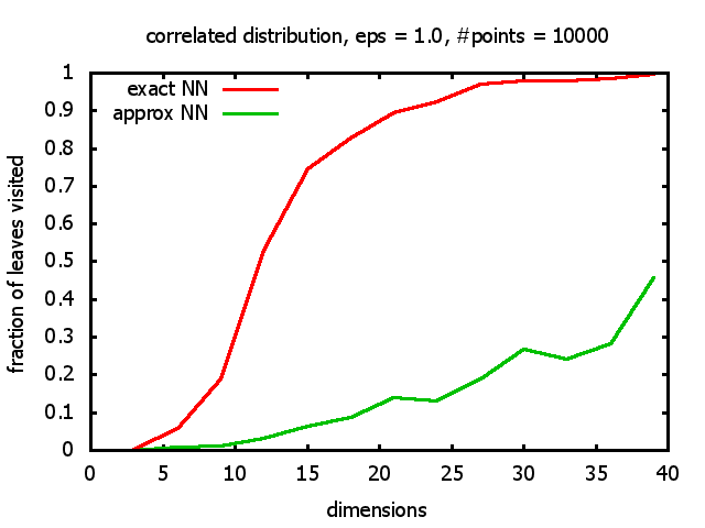
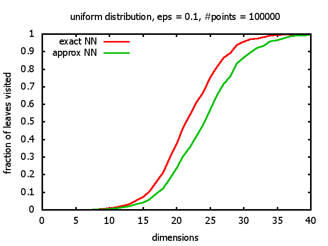
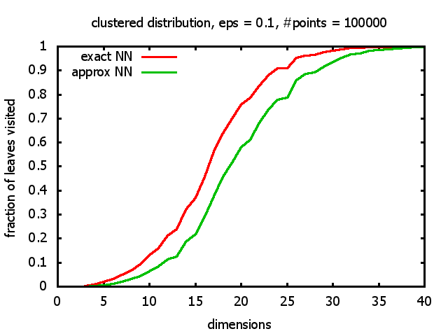
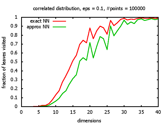
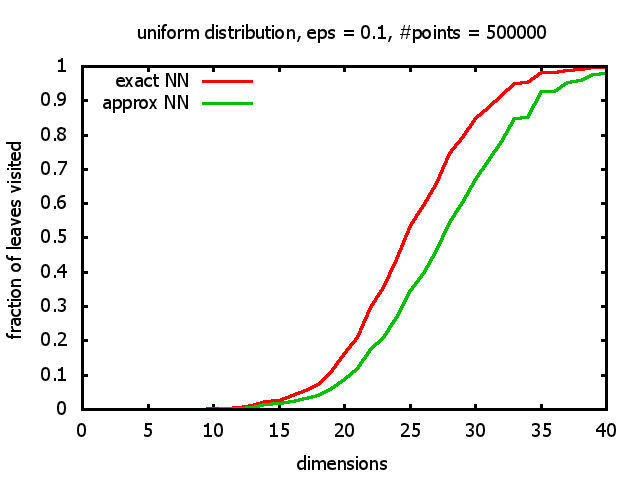
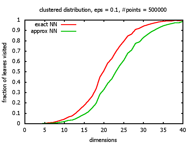
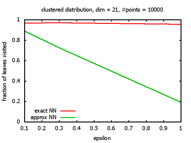
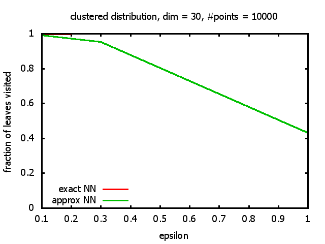
With each query, I have counted the number of leaves that the query algorithm visits. And finally, I have plotted the average number of leaves visited, depending on the dimension of the points.

The three distributions I have used are the following:
Uniform: each coordinate of each point is indipendently and identically distributed; the values are generated using Python's uniform random number generator.
Clustered: the set of points consists of a number of clusters; each cluster consists of 1000 points, each of which is distributed around a cluster center according to a normal distribution (sigma²=0.001); each cluster center is a random point that is generated using a uniform distribution.
Correlated: the set of points is created using an auto-correlation; the first point is randomly picked inside the unit cube; all following points are generated according to
     p_i+1 = 0.9 * p_i + 0.1 * w,
where p, w ∈ R^d,
and w is a "noise vector" from a Gaussian Distribution; after all points have been created, the whole set is scaled such that its bounding box equals the unit cube.
You can find more details about the distributions in the source code.

I believe, the results apply to the nearest neighbor search algorithms / kd-trees of CGAL as well.

Results

Performance = f(n), ε = 0.1, different dimensions, clustered distribution

Performance = f(d), 10k points, ε = 0.1, different distributions

Performance = f(d), 10k points, ε = 0.3, different distributions

Performance = f(d), 10k points, ε = 1.0, different distributions

Performance = f(d), 100k points, ε = 0.1, different distributions

Performance = f(d), 500k points, ε = 0.1, different distributions

Performance = f(ε), 10k points, different dimensions, clustered distribution

Downloads

It contains the Python program for building a kd-tree over a set of d-dimensional points and searching the nearest neighbor, and the approximate nearest neighbor. It contains also the same code again, but instrumented with some statistics gathering code. In addition, there is a Python class for d-dimensional vectors. And, finally, it contains all the shell scripts that I wrote for running the experiments (on a Linux cluster), and for plotting the results.

Contact